Learning About Learned Indices
Understanding the key results from Kraska et al. (2017) and ways to apply them to other domains.
By Elena Berman, Hashem Elezabi, Ankush Swarnakar, and Markie Wagner
Finding an index based on a key quickly is an immensely important task in computer science. In database systems, this task is critical. Years of research in this field have resulted in well-designed and efficient data structures such as B-trees, hash tables, and Bloom filters, which use indexing to determine the position of some object within some larger data structure, like an array.
These data structures are able to generalize and guarantee efficiency for data sets of any distribution. This is because what a B-tree, hash map, or any other index data structure does is structure the data in a way that works well in the general case, irrespective of specific properties of the data to be indexed. However, are there more efficient data structures if we know the structure of the underlying data?
Knowing properties of the data distribution can provide significant improvements in efficiency in an indexing structure. In a 2017 paper, computer science researchers proposed using modern machine learning (ML) methods, rather than traditional CS theory, to help computers learn how to use these structures, with the added benefit of capturing useful properties of the underlying data distribution. These methods use ML to take advantage of the data distribution in order to achieve greater efficiency. In light of recent developments in specialized hardware (like GPUs, TPUs, etc.) that enable us to train and run ML models ever-faster, this idea is well-aligned with the latest computing trends.
Distributions and Data Structures
What does it mean to “take advantage of the distribution”? It sounds like a really cool idea: our index structure can now tune itself to adapt to specific distributions of the input key data. But we haven’t made this concept concrete yet. So far, we have said that an ML model can be trained to take a key as input and output a position in the array. Let’s dive into what exactly that means with a few examples.
We start with a very simple example. Let’s say you have the following set of n keys, with n associated values (not shown here):
[0, 1, 2, 3, …, n –1]
We’d like to store these keys in sorted order, and we’d like to support lookups, insertions, and deletions. This is a natural task for a tree-based index, such as a balanced binary search tree (BST). In fact, the C++ std::map data structure is typically implemented using a red-black tree under the hood. In cases where the data don’t fit in memory, the B-tree structure is a very common choice and it’s used in many real-world database systems. For the purposes of this example, we’ll use a balanced BST. Assume n = 10, so that we have keys 0, 1, …, 9. If we insert these keys into a red-black tree one-by-one, we would get something like this:
Any operation on this red-black tree takes time O(log n). Now, do we really need to do this? For this particular set of keys, it seems overkill. Specifically, there is a certain structure to the keys that we are ignoring. In this case, the keys are all consecutive and start at 0. Building a binary search tree that searches the keys by splitting the search space each time until it finds the key is not necessary for these keys, given their simple structure. In fact, in this example, to access a key k we can simply go to position k in the array!
What we just saw is exactly what motivated the idea of learned indexes in the original paper by Kraska et. al. Instead of using a general-purpose index structure like a red-black tree, which is designed with no assumptions about the key distribution, we can use a learned index that can tailor itself to the key distribution. As we saw, if we know the data is an ascending list from 0 to 10, then we can more easily identify the location of each key. If we need to do insertions and deletions, things get more complicated, and update-able learned indexes are an active area of research. But for the static case, this example shows we can do much better just by knowing the distribution of the keys.
What if the keys are slightly more complicated? For example, say we have the keys [100, 101, 102, …, 100 + n –1]. Well, for a key k, we can simply map it to position k –100. If the keys are [100, 102, 104, …, 100 + 2(n –1)], then our mapped position would be (k –100) / 2. You get the idea.
The All-Powerful Cumulative Distribution Function
Let’s look more closely at the mappings we’ve been using to go from key to array position. One way to look at these functions is that they are approximating the cumulative distribution functions (CDFs) of the keys. Recall that the CDF of a random variable X is a function f(x) that gives the probability that X takes a value less than or equal to the input number x. In this case we are interested in approximating the empirical CDF of the keys. This just means we’re not dealing with a clean, analytical distribution described exactly by a mathematical random variable (if we are, even better!). To compute the empirical CDF of a dataset of keys, we can perform the following simple procedure. For each key, count the number of keys smaller than or equal to that key, and divide that number by the total number of keys to get a value between 0 and 1. This value is the cumulative density for that key. Now we can plot the keys on the x-axis and the cumulative density values on the y-axis.
If we use this procedure on the keys [0, 1, …, n] we get this plot:
This corresponds to the linear f(k) = k mentioned earlier. For the keys [100, 101, … ] we get this:
Notice that this corresponds to the expression we mentioned earlier: k — 100 (since the domain of keys starts at 100, the plot is shifted to the right by 100). Importantly, these distributions are toy examples that aren’t reflective of real-world scenarios. However, the exciting results from the past few years (e.g. here and here) have shown that the same idea works with more complicated distributions, including raw real-world data! The mappings that are learned to go from key to index are typically not straightforward copies of the empirical CDF like we’ve seen, but the intuition still holds. We discuss this further in the later sections, along with some techniques for dealing with more complex (or harder to learn) distributions.
The idea we just showed can be used to replace traditional indexes like B-trees, hash tables, and Bloom filters. The common theme is that we can use a model of the key distribution to build an index that is tailored to the input keys. That said, there are some differences between how we apply these ideas to different kinds of indexes, which we discuss more in-depth later.
In the case of learned index structures to replace hash tables and Bloom filters, the CDF function is used explicitly in the hash function definition. A hash function f that maps to a container with m buckets, it can simply scale the output: f(x) = m * CDF(x) in the case of the Bloom filter. To see how this occurs using the CDF in the example above, for key 600 where CDF(600) = 0.6, we’d have f(x) = 0.6m. If there are 1,000 buckets, we’d have f(x) = 600, exactly.
The Learning Process
Now that we see why knowing the approximate data distribution can be useful in building efficient indexing structures, let’s take a look at how a continuous function for the distribution can be learned in the first place. The authors of the 2017 paper used a unique model, which they called “Recursive Model Index” (RMI).
The core idea is to have several models that we can choose from in order to get our index from the key. In fact, we use a hierarchical approach to selecting model functions to take in a key and return an index. Instead of training one model to return values, the Recursive Model Index utilizes several layers of staged models. It is modeled as a B-tree. At a high level, the key is passed into the model at the “root” of the B-tree, and the model outputs which child-model to check next. The leaf nodes in this B-tree correspond to models that take in the key and output the actual position in the array.
Why is such a structure necessary? Why can’t we simply use one single learned function? The authors observed that when functions are approximated for real-world data sets, a function approximated at a high-level to describe the overall distribution is not accurate at a micro-level. For example, consider the picture below. Perhaps the function on the left has been approximated from a certain set of data points. However, when we look more closely, the distribution of some data points may not be captured accurately at a micro-level by the high-level function. The figure shows that a subset of the data appearing to follow an almost-linear distribution at a high-level actually may follow an exponential distribution.
We can decide before training how many “stages” of the model we would like to have. Each stage would be a layer in the B-tree of models, so a “1-stage” model would consist of one function which returns an index, whereas a “2-stage” model would consist of a function that would return which function to look at next, and the next function would return an index. Additionally, we can specify how many functions we want to have at each layer (besides the root layer).
Let’s say we have a set of n (key, index) pairs and we would like to obtain our model. We would recursively train our model from the “highest” level down. At the root-level, we can train a neural network which takes in a key and outputs an index. We then split up the dataset into sets that are the size of the number of functions per layer using the value that the trained function returns.
To illustrate this, let’s say that we’ve trained a top-level “root” model on a set of keys and values. The next step is to divide the data into the number of models we want at our next stage. This step works because the data is guaranteed to be in sorted order for a Range Index problem. In the 2017 paper, the authors do this by dividing the predicted-value set numbers into the number of stages. If the number of functions at the next step is 3, we would want to have three sets: set 0, set 1, and set 2 on which we would train the next 3 models respectively. We continue doing this for each level until we have our final model.
What is the connection between learned functions and simply using the CDF? In the 2017 paper, a key claim is that “continuous functions, describing the data distribution, can be used to build more efficient data structures or algorithms.” Thus, it is important to note that there are two distinct processes used: the first is to approximate models of continuous functions using machine learning and the Recursive Model Index, and the second is to approximate the CDF by counting the data distribution up-front. The first is used to replace B-Trees in index-lookup problems, and the second is used to replace hash functions in Hash Maps and Bloom Filters. Both learned models and CDFs fundamentally capture the data by modelling its distribution as a continuous function. The reason we learn a function for the first case is that we have (key, index) pairs in ascending order as our data type; however, in the second case, we only have the keys (which we know ahead of time). Thus, learning a function makes sense in the first case, but mapping the CDF exactly makes sense in the second case.
Error Bounds & Guarantees
Although B-Trees, HashTables, and Bloom Filters may not always return the correct answer for indexing problems, they offer strong guarantees on the types of errors they have that generalize across data distribution types. If we were searching for an index range, B-Trees guarantee a maximum error of the index’s page-size, while HashTables often have a low expected probability of element collision, depending on the type of hash function used. Bloom filters offer the strong guarantee of no false positives.
Can Learned Index structures offer the same kind of guarantees with any type of data distribution? To see this, let’s examine what happens if the RMI model for a B-tree has a higher error than the maximum page-size. After training our RMI hierarchy of functions, we calculate the absolute error, and find that it is higher than the highest possible error in a B-tree. What do we do next?
The authors of the 2017 paper solved this problem by using a Hybrid Index: a combination of Learned Index and B-Tree structures. If one subtree of the RMI does not perform within the guaranteed error bounds, we would replace that particular subtree with a B-tree constructed from the keys that would be predicted in that subtree.
And how can a Learned Index structure guarantee that there are no false positives? Using a neural network or other learned function sacrifices the guarantee that there are no false negatives provided by bloom filters. A simple solution the authors propose is to use a “spill-over” bloom filter if the model says a key is not in the set, which eliminates false negatives while being much smaller than a typical bloom filter due to its usage restricted to “hard” keys that the model can’t classify correctly.
Latest Work & Future Directions
How do Learned Index structures actually work in-practice? The latest performance results from several papers is shown below. In the original paper, the authors tested the structures on three data sets: 2 real-life datasets of maps and web data, and a constructed data set designed to follow a log-normal distribution, for the reason that it may be more difficult for the model to learn. Results, as shown in Table 1, showed promise.
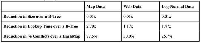
Results on the three datasets from the Bloom Filter were not reported; however, the authors suggested that a Bloom Filter with a false positive rate of 1% can be built with a 36% reduction in size.
Since the 2017 paper, other authors have studied this problem as well. In particular, verifying these results and creating an open source implementation of the RMI model has been an important area of research. More recently, researchers have investigated ways to update Learned Index structures with new data.
The RMI structure has shown remarkable promise in real-world data sets. Testing on datasets consisting of 200 million 64-bit integers from real-world datasets on Amazon sales, Facebook user ids, and open-source street map locations has demonstrated that the RMI structure is as good as, or outperforms, other structures in lookup time in nanoseconds (in a paper that creates a benchmark for Learned Index structures). However, it is still outperformed by FAST, a binary tree optimization from 2010, in terms of number of branch mispredictions and instructions executed, as well as build-time. RMI structures take a longer time to build than traditional B-Trees.
There are plenty of open problems associated with Learned Index structures: how can knowing the CDF speed up sorting and joins in a database? Are these structures extendable to multiple dimensions? These are important questions to follow in the future! We’re particularly interested in learning how the insights learned from the CDF may be useful in traditional data structures, and whether the performance increase from Machine Learning is actually the result of leveraging the CDF rather than from any properties of ML itself.
Bringing ML to Other Data Structures:
It’s easy to walk away from this paper and think: “Huh, ML can replace anything.” But what are the fundamental ideas that the authors introduced? While ML is ubiquitous throughout their work, two tangible takeaways are:
- Use data probability distributions to optimize data structures
- Use recursive models & auxiliary structures to optimize data structures
Let’s explore these ideas a bit further. The original paper focuses mainly on indexing structures, like B-Trees, Hash Maps, and Bloom Filters. Since we plan to investigate the effects of probability distributions on these structures, let’s take a deep-dive into a probabilistic structure instead — the Count-Min Sketch.
For side-by-side comparison with our analysis, we’ve implemented several of our experiments as interactive Python widgets here. We’ll also link directly to the exact simulations throughout this article in the captions for relevant figures. We deployed the visualization using NBInteract; just note that it might take a few seconds for the widgets to initialize on your page!
Simulating the Count-Min Sketch:
The Count-Min Sketch (described more fully here) is a data structure that can estimate the number of occurrences of discrete elements in a stream of data, without storing a unique counter for each distinct element.
At a high-level, the Sketch supports two core operations:
- count(el): records an occurrence of el in the data stream
- estimate(el): returns an estimate of the number of occurrences of el thus far
The Sketch provides a probabilistic bound on the estimation errors, using two hyper-parameters: ε (corresponds to the error tolerance) and 𝛿 (corresponds to the probability of intolerable errors). In particular, suppose you have a stream where all the true counts sum up to n. For any given element, let x denote the true count, and let x’ denote the estimated count. The Count-Min Sketch guarantees
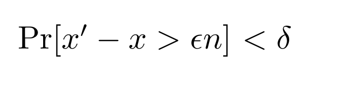
or intuitively, that the proportion of errors exceeding a “tolerable” error threshold (εn) is upper-bounded by 𝛿.
For further study, we’ve implemented a Count-Min-Sketch in Python, available here, as well as several variants to be used later. Our optimizations are largely inspired from the work of Vakilian, et al. at MIT CSAIL in 2019.
In a real-world scenario, a stream would consist of discrete elements that could take on many forms — integers (counts of values), hashes (codes), strings (search queries), etc. To simulate this appropriately, we feed our Count-Min Sketch with a set of integers, sampled from various probability distributions. Using integers guarantees that our inputs are discrete and allows us to create a one-to-one mapping between our simulated integer and a real-world data element.
Baseline Analysis:
Let’s start with a Count-Min Sketch with ε = 0.01 and 𝛿 = 0.05. Our data stream will consist of n = 10000 integers, sampled from a uniform distribution on [0, 1000]. The plot below shows the distribution of errors against their corresponding data points. Each blue point is an ordered pair of (error, data point) and the red line corresponds to the “tolerable error threshold” of εn = 100.
Average Error: 20.1535, Maximum Error: 76.0
Visually, we can tell the Count-Min Sketch is giving us decent estimates. The average error magnitude is fairly small and none of the errors exceed the threshold of 100.
What happens if we try different distributions? Consider a data stream of n = 10000 integers, sampled from a normal distribution with a mean of μ = 0 and standard deviation of σ = 100.
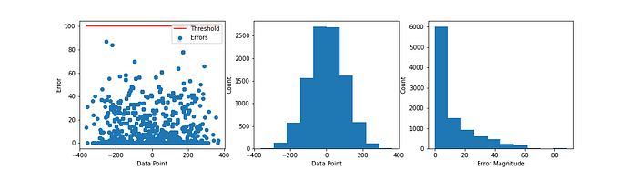
Average Error: 11.4482, Maximum Error: 88.0
The plot above shows the scatterplot of errors with data points (left), the distribution of data (center), and the distribution of errors (right). Again, we can see that the Count-Min Sketch gives us decent estimates; none of the errors exceed the threshold, which is excellent! But interestingly, by converting to a normal distribution, our average error almost halved, from 20.154 to 11.4482, and our max error shot up by 12.
Intuitively, this makes sense. In a uniform distribution, we would expect the counts of each element to be roughly equal. In turn, we can expect the errors for each element to also be roughly equal, since each error is a linear sum of counts. In normal distribution, the counts differ pretty significantly between different elements. In particular, elements with values closest to the mean of 0 are most common, and should have the highest counts. This means we do not expect the errors for each element to also be roughly equal. For example, when estimating the frequency of the most common elements, we are more likely to be off by a small amount relative to the true frequency, since the frequency of most other elements is small in comparison. However, if a small element shares all buckets with very frequent elements, we will see a significantly large error value.
To put this more concretely, let x be an element with a very low true count and let y be an element with a very high count; this means the count of x is much smaller than the count of y. If x and y are hashed into the same bucket, the estimated count of x is lower bounded by the true count of y, since estimating x returns the count of its bucket, which must contain the true count of y. In these cases, it’s easy to see why the error will be very high, because of the non-uniform distribution of counts.
However, though the maximum error is likely to increase, the average error is likely to decrease. As the distribution becomes more and more concentrated around a single value (in this case, the mean), the total number of discrete elements drops and the counts of the elements are roughly the same. This is doubly confirmed by the right-most plot in the figure above. The error distribution is heavily concentrated towards low errors, but has a tail that skews towards extremely high errors.
How does data spread affect our errors?
Let’s take this a step further and scope out the exact effect on standard deviation (a mathematical proxy for the “spread” of the data) on the errors. Let’s investigate what happens when we sample n = 1000 integers from a normal distribution with a mean of μ = 0. We vary the standard deviation between 1 and 100 to understand how spreading the distribution affects errors.
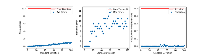
The figure above shows how average error (left), maximum error (center), and the proportion of intolerable errors (right) vary with standard deviation. Most interestingly, we see that as standard deviation increases, average error also increases. That means that the further we spread out our distribution, the higher average error we’re likely to see. Again, this makes sense — earlier we saw that the uniform distribution generally has higher average error than the normal distribution; “spreading” out the normal distribution makes it more like a uniform distribution.
We also see that generally, the maximum errors are higher for larger standard deviations. Intuitively, this is because with more spread out data, you’re likely to have very many elements with low counts, and less elements with high counts. This introduces more of the low-count-x-hashed-to-the-same-bucket-as-high-count-y problem we discussed earlier, which contributes to larger and larger error magnitudes in those cases.
Note: the last two graphs don’t illustrate a clear relationship between maximum error and the proportion of intolerable errors with respect to standard deviation, because this represents analysis conducted on 1 sampling of data from the normal distribution. If we were to average our values over many samples, we’d likely see a clearer trend. We focus on one sample in this writeup to explain the particularities of the errors to motivate further investigation.
Ultimately, we can conclude that the distribution of data does matter for the accuracies of our sketches. So let’s try to optimize Count-Min Sketches with this in mind.
Optimization #1: The Learned Count-Min Sketch
Earlier, we discussed how “extreme errors” are induced when you have elements with drastically different counts hashed to the same bucket. Distinguishing between high-count elements and low-count elements isn’t exactly a novel idea on data structures designed for data streams. In fact, computer scientists often call these high-frequency elements (with high-counts) “Heavy Hitters”. Our analysis demonstrates that heavy hitters colliding with non-heavy-hitters produces large errors. How can we avoid this?
One approach is simply to treat the heavy hitters and non-heavy-hitters separately. This is where we can motivate our data structure design with two ideas from the original Learned Index Structures paper — recursive models and auxiliary structures.
Instead of storing heavy hitters in the sketch, let’s instead initialize an auxiliary hash table that stores the exact counts of the heavy hitters. This means each element that is a heavy hitter will get its own unique bucket to keep track of only that element’s count, guaranteeing that the error for estimating the count of that particular element is 0. For non heavy-hitter elements, we simply store them in a Count-Min-Sketch as before.
How do we distinguish between heavy hitters and non-heavy-hitters computationally? We know the probability distribution of the data! So we know which elements are “most likely” (highest counts) and which ones are “least likely” (lowest counts). We can leverage ML to train a binary classifier to distinguish between these “most likely” and “least likely” elements. We call this binary classifier an “oracle”.
In our particular implementation, we use a 2-layer neural network with hidden layers of size 30 and 40 respectively, trained with softmax loss and vanilla stochastic gradient descent for a maximum of 500 iterations. In practice, we should set this classifier to the “most applicable” to the data set and data distribution — it could be an SVM, logistic regression, neural network, k-Nearest Neighbors, or anything else.
Graphically, we can visualize our new data structure as follows:
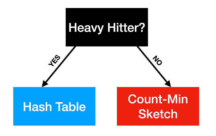
Observe that by introducing an auxiliary structure (hash table) with an oracle (which answers the heavy hitter question), we’ve built a recursive model, much like the Bloom Filter from the original Learned Index Paper. As we move forward, let’s call this new data structure a “Learned Count Min Sketch.”
How does this perform in practice? Let’s compare our Regular Count-Min Sketch with our Learned Count-Min Sketch on n = 1000 data points, sampled from a uniform distribution on [0, 1000] with ε = 0.01 and 𝛿 = 0.05.
Regular Count-Min Sketch: Average Error: 1.592, Maximum Error: 7.0
Learned Count-Min Sketch: Average Error: 1.588, Maximum Error: 7.0
Interestingly, the error distributions almost look the same! The learned sketch’s average error is a hair lower than the regular sketch, but not enough to conclude anything significant.
Why is the case? Let’s again think back to the idea of the heavy hitter. In a uniform distribution, we expect all the counts to roughly be the same — meaning in theory, there should be no heavy hitters! Our classifier is classifying most elements as non-heavy-hitters, which means that most of the data still is being processed by the regular count-min sketch embedded within the learned sketch. And thus, we see the errors are likely to be the same.
Now, let’s try with a distribution that does have heavy hitters — the normal distribution. Our data is now n = 1000 integers, sampled from a normal distribution with a μ = 0 and standard deviation of σ = 100. We choose ε = 0.01 and 𝛿 = 0.05 for both our sketches.
Regular Count-Min Sketch: Average Error: 1.027, Maximum Error: 13.0
Learned Count-Min Sketch: Average Error: 0.248, Maximum Error: 7.0
Promising results! Our average error is more than 4 times smaller and our maximum error is halved by using the learned count-min sketch. We also see that the error distribution for the learned count-min sketch has much more of the mass towards 0, meaning errors are generally smaller.
Optimization #2: Rules Count-Min Sketch
Let’s take it a step even further. Why do we need machine-learning anyways? What if we know the data distribution so well that we know exactly which elements are going to be heavy hitters?
Suppose you’re Jeff Dean on a regular Tuesday afternoon and you think to yourself — “I wonder what are the frequencies of different search queries on Google for 2020!” Maybe you have data from 2019 on the most frequent search terms. You know 2020 data is likely to be close to that of 2019 (barring a pandemic, among other things :/), so you treat the most frequent queries from 2019 as heavy hitters. Instead of learning what the heavy-hitters are, we use a rules-based approach.
How do we simulate this concept without using ML? Fundamentally, any rules-based approach for determining will give a yes/no answer to whether a given element is a heavy hitter. To emulate this, we can construct a set of data points that will be heavy hitters based on “rules.” Our “rule” is: if the element is within the top p proportion of counts in the data set, it’s a heavy hitter. Real-world applications will have different rules! This is simply a proxy for the “most common” elements. The point is to switch from our ML approach to a more deterministic approach. We can thus iterate through our data set, add all heavy-hitters to a set, and then feed that set into our sketch constructor. Now, instead of inferring whether an element is a heavy hitter, we can simply check its presence within our set.
Again, we experiment on n = 1000 integers, sampled from a normal distribution with a mean of 0 and a standard deviation of 100. We choose ε = 0.01 and 𝛿 = 0.05 for both our sketches. We also choose the top p = 0.2 proportion of elements to be characterized as “heavy-hitters.”
Regular Count-Min Sketch: Average Error: 0.89, Maximum Error: 12.0
Rule Count-Min Sketch: Average Error: 0.279, Maximum Error: 6.0
Even when we eliminate ML, we can reduce the average error to a third of the regular average error, and halve the maximum error. This is huge, because it demonstrates that knowledge of the probability distribution is itself enough to optimize a data structure.
Let’s finally investigate what happens as we change the tolerance for what we consider to be a heavy hitter. Currently, we designate an element as a heavy hitter if its true count is in the top p proportion of all counts, where p = 0.2. Let’s now vary p between 0 and 1, and see what that gets us.
The average error seems to decrease exponentially with increasing p. Intuitively, this makes sense, as with larger p, more elements are stored in the unique hash table with exact counts, meaning fewer incorrect estimates. Trivially, when p = 1, all the elements are stored in the unique hash table, so the average error must be 0. Wouldn’t it be nice if we always had enough space for that?
Final Thoughts
All in all, what can we conclude? We leveraged two ideas from the original Learned Index Paper (probability distribution optimization &recursive models) and applied them towards the Count-Min Sketch data structure. In reality, optimizing them was fairly simple (check out the implementation for yourself!). What we’ve constructed is similar to the idea of a cache in read-write data structures (like B-Trees). Instead of optimizing for the speed of the most accurate elements, we optimize their accuracy. All we need is an oracle to tell us if an element is a heavy hitter (which can be implemented via ML, or other means) and an auxiliary hash table to store exact counts of heavy hitters.
Machine learning is a very powerful tool, but that’s all it is — a tool. Like we mentioned earlier, the takeaway from the original paper isn’t necessarily to aggressively replace everything with ML. Rather, it suggests that we use ML as a tool in optimizing data structures. Simple optimizations, made possible with knowledge of probability distributions via ML, can produce huge advantages in speed, as seen in the original work, and accuracy, as demonstrated here.
If you’ve made it this far, congrats and thanks for sticking through! We hoped you learned a thing or two about ML in data structures. We also want to shout out our CS166 instructor Keith Schwarz and TAs Anton de Leon & Ryan Smith for a phenomenal quarter!
Further Reading:
- The original 2017 paper.
- Seminar: Authors on their paper.
- The Case for Learned Index Structures Medium post
- Benchmark for Learned Index Structures paper
- Open-Source Implementation of RMI structure.
- ALEX: An Updatable Adaptive Learned Index
All figures in paper were made by authors unless otherwise noted.